Inspecting the results of processing#
After running the entire pipeline, you should have all results under the output/results/ folder.
CSA for T2 data#
Here for example, we show the mean CSA averaged between C2-C3 levels computed from the T2 data. Each line represents a subject.
Filename |
Slice (I->S) |
VertLevel |
MEAN(area) |
STD(area) |
|---|---|---|---|---|
sub-01_T2w_seg.nii.gz |
161:203 |
2:3 |
83.5690681039387 |
2.82182217691781 |
sub-03_T2w_seg.nii.gz |
159:199 |
2:3 |
60.6215201725797 |
2.87402688226702 |
sub-05_T2w_seg.nii.gz |
159:190 |
2:3 |
68.763579167899 |
3.19840203029727 |
The variability is mainly due to the inherent variability of CSA across subjects.
MTR in white matter#
Here are the results of MTR quantification in the dorsal column of each subject between C2 and C5. Notice the remarkable inter-subject consistency.
Filename |
Slice (I->S) |
VertLevel |
Label |
Size [vox] |
MAP() |
STD() |
|---|---|---|---|---|---|---|
sub-01/anat/mtr.nii.gz |
3:16 |
2:5 |
dorsal columns |
370.15204844543 |
49.7198531140872 |
4.99870360243909 |
sub-03/anat/mtr.nii.gz |
3:15 |
2:5 |
dorsal columns |
282.686966627213 |
49.3521578793729 |
5.19981366995629 |
sub-05/anat/mtr.nii.gz |
4:13 |
2:5 |
dorsal columns |
229.620127825366 |
49.2113270517532 |
4.76773091479419 |
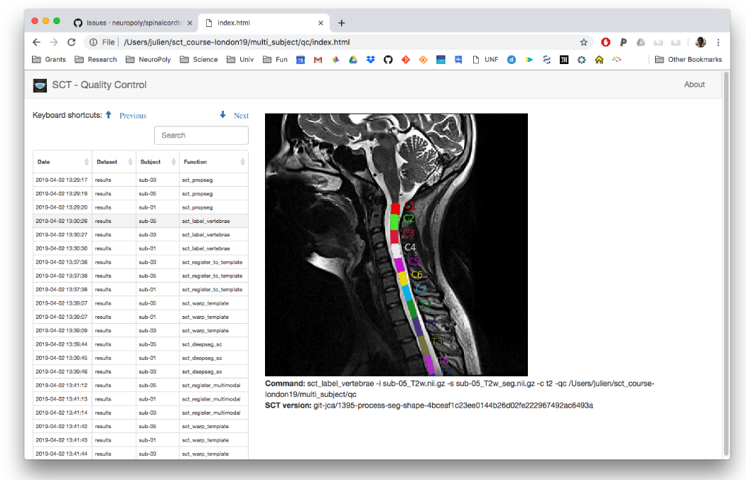
Quality Control report#
A QC report is generated under qc/. As shown before, the QC report is useful to quickly assess the quality of the analysis pipeline.