sct_deepseg_sc

Command-line usage

Spinal Cord Segmentation using convolutional networks. Reference: Gros et al. Automatic segmentation of the spinal cord and intramedullary multiple sclerosis lesions with convolutional neural networks. Neuroimage. 2019 Jan 1;184:901-915.

usage: sct_deepseg_sc -i <file> -c {t1,t2,t2s,dwi}
                      [-centerline {svm,cnn,viewer,file}]
                      [-file_centerline <str>] [-thr <float>] [-brain {0,1}]
                      [-kernel {2d,3d}] [-ofolder <str>] [-o <file>] [-qc <str>]
                      [-qc-dataset <str>] [-qc-subject <str>] [-h] [-v <int>]
                      [-profile-time [<file>]] [-trace-memory [<folder>]]
                      [-r {0,1}]

MANDATORY ARGUMENTS

-i

Input image. Example: t1.nii.gz

-c

Possible choices: t1, t2, t2s, dwi

Type of image contrast.

OPTIONAL ARGUMENTS

-centerline

Possible choices: svm, cnn, viewer, file

Method used for extracting the centerline:

• svm: Automatic detection using Support Vector Machine algorithm.

• cnn: Automatic detection using Convolutional Neural Network.

• viewer: Semi-automatic detection using manual selection of a few points with an interactive viewer followed by regularization.

• file: Use an existing centerline (use with flag -file_centerline)

Default: “svm”

-file_centerline

Input centerline file (to use with flag -centerline file). Example: t2_centerline_manual.nii.gz

-thr

Binarization threshold (between 0 and 1) to apply to the segmentation prediction. Set to -1 for no binarization (i.e. soft segmentation output). The default threshold is specific to each contrast and was estimated using an optimization algorithm. More details at: https://github.com/sct-pipeline/deepseg-threshold.

-brain

Possible choices: 0, 1

Indicate if the input image contains brain sections (to speed up segmentation). Only use with -centerline cnn. (default: 1 for T1/T2 contrasts, 0 for T2*/DWI contrasts)

-kernel

Possible choices: 2d, 3d

Choice of kernel shape for the CNN. Segmentation with 3D kernels is slower than with 2D kernels.

Default: “2d”

-ofolder

Output folder.

Default: “/home/docs/checkouts/readthedocs.org/user_builds/spinalcordtoolbox/checkouts/stable/documentation/source”

-o

Output filename. Example: spinal_seg.nii.gz

-qc

The path where the quality control generated content will be saved

-qc-dataset

If provided, this string will be mentioned in the QC report as the dataset the process was run on

-qc-subject

If provided, this string will be mentioned in the QC report as the subject the process was run on

MISC ARGUMENTS

-v

Possible choices: 0, 1, 2

Verbosity. 0: Display only errors/warnings, 1: Errors/warnings + info messages, 2: Debug mode.

Default: 1

-profile-time

Enables time-based profiling of the program, dumping the results to the specified file.

If no file is specified, human-readable results are placed into a ‘time_profiling_results.txt’ document in the current directory (’/home/docs/checkouts/readthedocs.org/user_builds/spinalcordtoolbox/checkouts/stable/documentation/source’). If the specified file is a .prof file, the file will instead be in binary format, ready for use with common post-profiler utilities (such as snakeviz).

-trace-memory

Enables memory tracing of the program.

When active, a measure of the peak memory (in KiB) will be output to the file peak_memory.txt. Optionally, developers can also modify the SCT code to add additional snapshot_memory() calls. These calls will ‘snapshot’ the memory usage at that moment, saving the memory trace at that point into a second file (memory_snapshots.txt).

By default, both outputs will be placed in the current directory (’/home/docs/checkouts/readthedocs.org/user_builds/spinalcordtoolbox/checkouts/stable/documentation/source’). Optionally, you may provide an alternative directory (-trace-memory <dir_name>), in which case all files will be placed in that directory instead. Note that this WILL incur an overhead to runtime, so it is generally advised that you do not run this in conjunction with the time profiler or in time-sensitive contexts.

-r

Possible choices: 0, 1

Remove temporary files.

Default: 1

Algorithm details

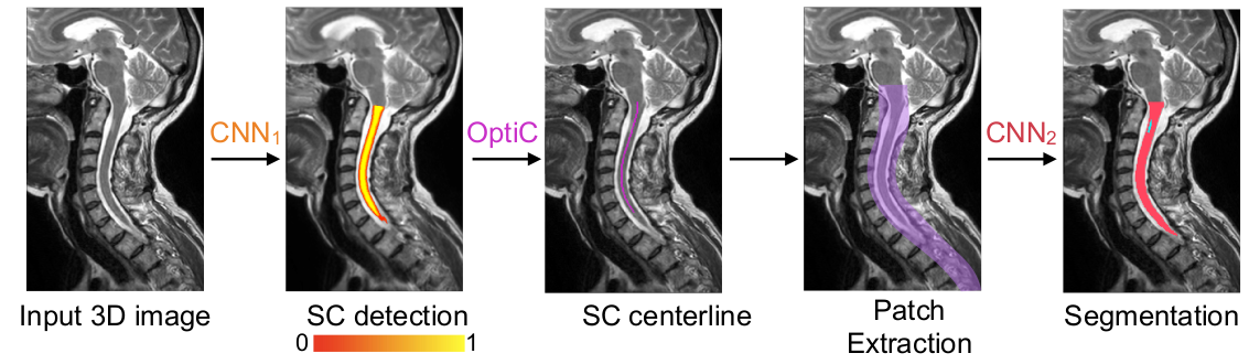
As its name suggests, sct_deepseg_sc is based on deep learning. It is a newer algorithm, having been introduced to SCT in 2018. The steps of the algorithm are as follows:

1. Spinal cord detection

First, a convolutional neural network is used to generate a probablistic heatmap for the location of the spinal cord.

2. Centerline detection

The heatmap is then fed into the OptiC algorithm to detect the spinal cord centerline.

3. Patch extraction

The spinal cord centerline is used to extract a patch from the image. (This is done to exclude regions that we are certain do not contain the spinal cord.)

4. Segmentation

Lastly, a second convolutional neural network is applied to the extracted patch to segment the spinal cord.

Fixing a failed sct_deepseg_sc segmentation

Due to contrast variations in MR imaging protocols, the contrast between the spinal cord and the cerebro-spinal fluid (CSF) can differ between MR volumes. Therefore, the segmentation method may fail sometimes in presence of artifacts, low contrast, etc.

You have several options if the segmentation fails:

• Change the kernel size from 2D to 3D using the -kernel argument.

• Change the centerline detection method using the -centerline argument.

• Try the newest segmentation method that is robust to many contrasts: (sct_deepseg)

• Try the legacy segmentation method based on mesh propagation: (sct_propseg)

• Check the specialized models in sct_deepseg to see if one fits your use case.

• Manually correct the segmentation.

• Ask for help on the SCT forum.