sct_propseg

Command-line Help

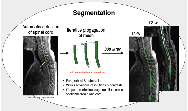
This program segments automatically the spinal cord on T1- and T2-weighted images, for any field of view. You must provide the type of contrast, the image as well as the output folder path. The segmentation follows the spinal cord centerline, which is provided by an automatic tool: Optic. The initialization of the segmentation is made on the median slice of the centerline, and can be adjusted using the -init parameter. The initial radius of the tubular mesh that will be propagated should be adapted to size of the spinal cord on the initial propagation slice.

Primary output is the binary mask of the spinal cord segmentation. This method must provide VTK triangular mesh of the segmentation (option -mesh). Spinal cord centerline is available as a binary image (-centerline-binary) or a text file with coordinates in world referential (-centerline-coord).

Cross-sectional areas along the spinal cord can be available (-cross). Several tips on segmentation correction can be found on the ‘Correcting sct_propseg’ page in the Tutorials section of the documentation.

If the segmentation fails at some location (e.g. due to poor contrast between spinal cord and CSF), edit your anatomical image (e.g. with fslview) and manually enhance the contrast by adding bright values around the spinal cord for T2-weighted images (dark values for T1-weighted). Then, launch the segmentation again.

References:

• De Leener B, Kadoury S, Cohen-Adad J. Robust, accurate and fast automatic segmentation of the spinal cord. Neuroimage 98, 2014. pp 528-536. DOI: 10.1016/j.neuroimage.2014.04.051

• De Leener B, Cohen-Adad J, Kadoury S. Automatic segmentation of the spinal cord and spinal canal coupled with vertebral labeling. IEEE Trans Med Imaging. 2015 Aug;34(8):1705-18.

usage: sct_propseg -i <file> -c {t1,t2,t2s,dwi} [-o <file>] [-ofolder <folder>]
                   [-down <int>] [-up <int>] [-mesh] [-centerline-binary] [-CSF]
                   [-centerline-coord] [-cross] [-init-tube]
                   [-low-resolution-mesh] [-init-centerline <file>]
                   [-init <float>] [-init-mask <file>] [-mask-correction <file>]
                   [-rescale <float>] [-radius <float>] [-nbiter <int>]
                   [-max-area <float>] [-max-deformation <float>]
                   [-min-contrast <float>] [-d <float>]
                   [-distance-search <float>] [-alpha <float>] [-qc <folder>]
                   [-qc-dataset <str>] [-qc-subject <str>] [-correct-seg <int>]
                   [-h] [-v <int>] [-profile-time [<file>]]
                   [-trace-memory [<folder>]] [-r {0,1}]

MANDATORY ARGUMENTS

-i

Input image. Example: ti.nii.gz

-c

Possible choices: t1, t2, t2s, dwi

Type of image contrast. If your contrast is not in the available options (t1, t2, t2s, dwi), use t1 (cord bright / CSF dark) or t2 (cord dark / CSF bright)

OPTIONAL ARGUMENTS

-o

Output filename. Example: spinal_seg.nii.gz

-ofolder

Output folder.

-down

Down limit of the propagation. Default is 0.

-up

Up limit of the propagation. Default is the highest slice of the image.

-mesh

Output: mesh of the spinal cord segmentation

Default: False

-centerline-binary

Output: centerline as a binary image.

Default: False

-CSF

Output: CSF segmentation.

Default: False

-centerline-coord

Output: centerline in world coordinates.

Default: False

-cross

Output: cross-sectional areas.

Default: False

-init-tube

Output: initial tubular meshes.

Default: False

-low-resolution-mesh

Output: low-resolution mesh.

Default: False

-init-centerline

Filename of centerline to use for the propagation. Use format .txt or .nii; see file structure in documentation.

Replace filename by viewer to use interactive viewer for providing centerline. Example: -init-centerline viewer

-init

Axial slice where the propagation starts, default is middle axial slice.

-init-mask

Mask containing three center of the spinal cord, used to initiate the propagation.

Replace filename by viewer to use interactive viewer for providing mask. Example: -init-mask viewer

-mask-correction

mask containing binary pixels at edges of the spinal cord on which the segmentation algorithm will be forced to register the surface. Can be used in case of poor/missing contrast between spinal cord and CSF or in the presence of artefacts/pathologies.

-rescale

Rescale the image (only the header, not the data) in order to enable segmentation on spinal cords with dimensions different than that of humans (e.g., mice, rats, elephants, etc.). For example, if the spinal cord is 2x smaller than that of human, then use -rescale 2

Default: 1.0

-radius

Approximate radius (in mm) of the spinal cord. Default is 4.

-nbiter

Stop condition (affects only the Z propogation): number of iteration for the propagation for both direction. Default is 200.

-max-area

[mm^2], stop condition (affects only the Z propogation): maximum cross-sectional area. Default is 120.

-max-deformation

[mm], stop condition (affects only the Z propogation): maximum deformation per iteration. Default is 2.5

-min-contrast

[intensity value], stop condition (affects only the Z propogation): minimum local SC/CSF contrast, default is 50

-d

trade-off between distance of most promising point (d is high) and feature strength (d is low), default depend on the contrast. Range of values from 0 to 50. 15-25 values show good results. Default is 10.

-distance-search

maximum distance of optimal points computation along the surface normals. Range of values from 0 to 30. Default is 15

-alpha

Trade-off between internal (alpha is high) and external (alpha is low) forces. Range of values from 0 to 50. Default is 25.

-qc

The path where the quality control generated content will be saved.

-qc-dataset

If provided, this string will be mentioned in the QC report as the dataset the process was run on.

-qc-subject

If provided, this string will be mentioned in the QC report as the subject the process was run on.

-correct-seg

Possible choices: 0, 1

Enable (1) or disable (0) the algorithm that checks and correct the output segmentation. More specifically, the algorithm checks if the segmentation is consistent with the centerline provided by isct_propseg.

Default: 1

MISC ARGUMENTS

-v

Possible choices: 0, 1, 2

Verbosity. 0: Display only errors/warnings, 1: Errors/warnings + info messages, 2: Debug mode.

Default: 1

-profile-time

Enables time-based profiling of the program, dumping the results to the specified file.

If no file is specified, human-readable results are placed into a ‘time_profiling_results.txt’ document in the current directory (’/home/docs/checkouts/readthedocs.org/user_builds/spinalcordtoolbox/checkouts/stable/documentation/source’). If the specified file is a .prof file, the file will instead be in binary format, ready for use with common post-profiler utilities (such as snakeviz).

-trace-memory

Enables memory tracing of the program.

When active, a measure of the peak memory (in KiB) will be output to the file peak_memory.txt. Optionally, developers can also modify the SCT code to add additional snapshot_memory() calls. These calls will ‘snapshot’ the memory usage at that moment, saving the memory trace at that point into a second file (memory_snapshots.txt).

By default, both outputs will be placed in the current directory (’/home/docs/checkouts/readthedocs.org/user_builds/spinalcordtoolbox/checkouts/stable/documentation/source’). Optionally, you may provide an alternative directory (-trace-memory <dir_name>), in which case all files will be placed in that directory instead. Note that this WILL incur an overhead to runtime, so it is generally advised that you do not run this in conjunction with the time profiler or in time-sensitive contexts.

-r

Possible choices: 0, 1

Remove temporary files.

Default: 1

Algorithm details

The sct_propseg algorithm is a three step process defined as follows:

1. Centerline detection

sct_propseg starts by using a machine learning-based method (OptiC) to automatically detect the approximate center of the spinal cord.

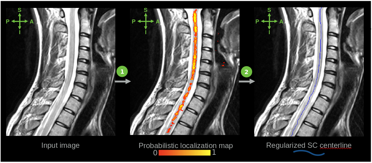
(The centerline detection step is also provided in a standalone script called sct_get_centerline.)

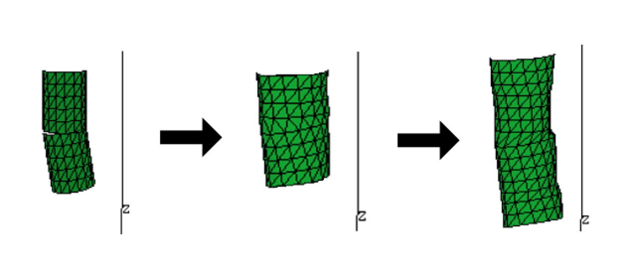
2. Mesh propagation

Next, a coarse 3D mesh is created by propagating along the spinal cord (PropSeg).

3. Surface refinement

Finally, the surface of the mesh is refined using small adjustments.

When to use sct_propseg

When choosing between sct_propseg and sct_deepseg spinalcord, it is important to know that no one algorithm is strictly superior in all cases; whether one works better than the other is data-dependent.

As a rule of thumb:

• sct_deepseg will generally perform better on “real world” scans of adult humans, including both healthy controls and subjects with conditions such as multiple sclerosis (MS), degenerative cervical myelopathy (DCM), and others. This is because sct_deepseg was trained on human subjects, including those with a range of common and representative spinal cord pathologies.

• sct_propseg, on the other hand, will generally perform better on non-standard scans, including exvivo spinal cords, pediatric subjects, and non-human species. This is because sct_propseg uses a mesh propagation-based approach that is more agnostic to details such as the shape and size of the spinal cord, the presence of surrounding tissue, etc.

That said, given the variation in imaging data (imaging centers, sizes, ages, coil strengths, contrasts, scanner vendors, etc.), SCT recommends to try both algorithms with your pilot scans to evaluate the merit of each on your specific dataset, then stick with a single method throughout your study.

Note: Development of these approaches is an iterative process, and the data used to develop these approaches evolves over time. If you have input regarding what has worked (or hasn’t worked) for you, we would be happy to hear your thoughts in the SCT forum, as it could help to improve the toolbox for future users.