Inspecting the results of processing¶

After running the entire pipeline, you should have all results under the output/results/ folder.

CSA for T2 data¶

Here for example, we show the mean CSA averaged between C2-C3 levels computed from the T2 data. Each line represents a subject.

`CSA.csv`: CSA values in T2 data across 3 subjects¶
Filename	Slice (I->S)	VertLevel	MEAN(area)	STD(area)
sub-01_T2w_seg.nii.gz	161:203	2:3	83.5690681039387	2.82182217691781
sub-03_T2w_seg.nii.gz	159:199	2:3	60.6215201725797	2.87402688226702
sub-05_T2w_seg.nii.gz	159:190	2:3	68.763579167899	3.19840203029727

The variability is mainly due to the inherent variability of CSA across subjects.

MTR in white matter¶

Here are the results of MTR quantification in the dorsal column of each subject between C2 and C5. Notice the remarkable inter-subject consistency.

`MTR_in_DC.csv`: MTR values values in white matter (dorsal columns) across 3 subjects¶
Filename	Slice (I->S)	VertLevel	Label	Size [vox]	MAP()	STD()
sub-01/anat/mtr.nii.gz	3:16	2:5	dorsal columns	370.15204844543	49.7198531140872	4.99870360243909
sub-03/anat/mtr.nii.gz	3:15	2:5	dorsal columns	282.686966627213	49.3521578793729	5.19981366995629
sub-05/anat/mtr.nii.gz	4:13	2:5	dorsal columns	229.620127825366	49.2113270517532	4.76773091479419

Quality Control report¶

Because the -qc flag was used for each of the SCT commands within the process_data.sh batch script, a QC report is generated under the qc/ folder. It can be viewed by running open qc/index.html, or by double-clicking on the index.html file:

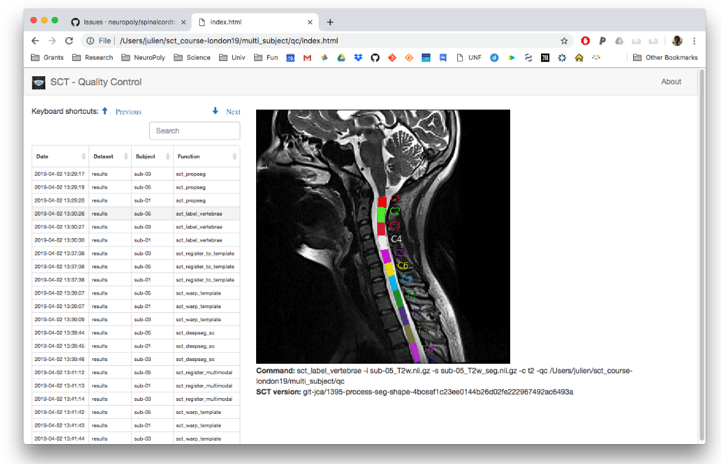
https://raw.githubusercontent.com/spinalcordtoolbox/doc-figures/master/batch-processing-of-subjects/qc.png

When processing multiple subjects (e.g., using sct_run_batch), QC reports are especially useful as they have several features to help quickly assess multiple images all at once:

The columns of the QC report can be sorted. For example, you can sort by “Function” to review the sct_deepseg outputs for all of the subjects together, then all of the sct_label_vertebrae outputs, and so on.
You can also use keyboard shortcuts to quickly skim through subjects. The arrow keys can be used to switch subjects and toggle the overlay, while the ‘F’ key can be used to mark subjects as “Fail”, “Artifact”, or “Pass”.
You can then use the “Export Fails” button to export failing subjects as a qc_fail.yml file, to be used alongside SCT’s manual correction scripts.

On the following page, we will see how to make use of this qc_fail.yml file for manual correction.

Note

For a deeper look at QC report features, you can also refer to the Quality Control (QC) Reports section of the Inspecting the results of your analysis (Quality Control, FSLeyes) page.