Cross-sectional area (CSA)
This section demonstrates how to compute spinal cord cross-sectional area.
Important
There is a limit to the precision you can achieve for a given image resolution. SCT does not truncate spurious digits when performing angle correction, so please keep in mind that there may be non-significant digits in the computed values. You may wish to compare angle-corrected values with their corresponding uncorrected values (-angle-corr 0) to get a sense of the limits on precision.
CSA (Averaged across vertebral levels)
First, we will start by computing the cord cross-sectional area (CSA) averaged across vertebral levels. As an example, we’ll choose the C3 and C4 vertebral levels, but you can specify any levels that are covered by the appropriate inferior/superior disc labels present in your disc label file.
sct_process_segmentation -i t2_seg.nii.gz -vert 3:4 -discfile t2_totalspineseg_discs.nii.gz -o csa_c3c4.csv
- Input arguments:
-i: The input segmentation file.-vert: The vertebral levels to compute metrics across. Vertebral levels can be specified individually (3,4) or as a range (3:4).-discfile: Disc label file used to map slices to vertebral levels. Here, we use labels generated by spine.-o: The output CSV file.
- Output files/folders:
csa_c3c4.csv: A file containing the CSA values and other shape metrics. This file is partially replicated in the table below.
Filename |
Slice (I->S) |
VertLevel |
MEAN(area) |
STD(area) |
|---|---|---|---|---|
single_subject/data/t2/t2_seg.nii.gz |
145:189 |
3:4 |
72.7770002120008 |
2.031463810597592 |
CSA (Per level)
Next, we will compute CSA for each individual vertebral level (rather than averaging), as well as introducing a new flag (-anat) to compute symmetry metrics.
sct_process_segmentation -i t2_seg.nii.gz -anat t2.nii.gz -vert 3:4 -discfile t2_totalspineseg_discs.nii.gz -perlevel 1 -o csa_perlevel.csv
- Input arguments:
-i: The input segmentation file.-anat: A corresponding anatomical file, used to compute symmetry metrics.-vert: The vertebral levels to compute metrics across. Vertebral levels can be specified individually (3,4) or as a range (3:4).-discfile: Disc label file used to map slices to vertebral levels.-perlevel: Set this option to 1 to turn on per-level computation.-o: The output CSV file.
- Output files/folders:
csa_perlevel.csv: A file containing the CSA values and other shape metrics. This file is partially replicated in the table below.
Filename |
Slice (I->S) |
VertLevel |
MEAN(area) |
STD(area) |
|---|---|---|---|---|
single_subject/data/t2/t2_seg.nii.gz |
145:168 |
4 |
73.29174144798469 |
2.236378671124064 |
single_subject/data/t2/t2_seg.nii.gz |
169:189 |
3 |
71.14226547373525 |
2.061192954901401 |
CSA (Per axial slice)
Finally, to compute CSA for individual slices, set the -perslice argument to 1, and use -z argument to specify axial slice numbers or a range of slices. (For slice numbering, 0 represents the slice furthest towards the inferior direction.)
sct_process_segmentation -i t2_seg.nii.gz -z 30:35 -discfile t2_totalspineseg_discs.nii.gz -perslice 1 -o csa_perslice.csv
- Input arguments:
-i: The input segmentation file.-perslice: Set this option to 1 to turn on per-slice computation.-z: The Z-axis slices to compute metrics for. Slices can be specified individually (30,31,32,33,34,35) or as a range (30:35).-discfile: Disc label file used to report vertebral-level correspondence for each slice.-o: The output CSV file.
- Output files/folders:
csa_perslice.csv: A file containing the CSA values and other shape metrics. This file is partially replicated in the table below.
Filename |
Slice (I->S) |
VertLevel |
MEAN(area) |
STD(area) |
|---|---|---|---|---|
single_subject/data/t2/t2_seg.nii.gz |
30 |
10 |
38.82506256917984 |
0.0 |
single_subject/data/t2/t2_seg.nii.gz |
31 |
10 |
38.199326002704446 |
0.0 |
single_subject/data/t2/t2_seg.nii.gz |
32 |
10 |
36.95834151629827 |
0.0 |
single_subject/data/t2/t2_seg.nii.gz |
33 |
10 |
38.18167628876984 |
0.0 |
single_subject/data/t2/t2_seg.nii.gz |
34 |
10 |
40.02060465413577 |
0.0 |
single_subject/data/t2/t2_seg.nii.gz |
35 |
9 |
37.55018351008499 |
0.0 |
CSA (PMJ-based)
Although using vertebral levels as a reference to compute CSA gives an approximation of the spinal levels, a drawback of that method is that it doesn’t consider neck flexion and extension (Cadotte et al., 2015).
To overcome this limitation, the CSA can instead be computed as a function of the distance to a neuroanatomical reference point. Here, we use the pontomedullary junction (PMJ) as a reference for computing CSA, since the distance from the PMJ along the spinal cord will vary depending on the position of the neck.
Computing the PMJ-based CSA involves a 4-step process (Bedard & Cohen-Adad, 2022):
The PMJ is detected using sct_detect_pmj.
The spinal cord centerline is extracted using a segmentation of the spinal cord, then the centerline is extended to the position of the PMJ label using linear interpolation and smoothing.
A mask is determined using two parameters: (1) distance along the centerline from the PMJ label, and (2) extent of the mask.
The CSA is computed and averaged within this mask.
For this tutorial, we will compute CSA at a distance of 64 mm from the PMJ using a mask with a 30 mm extent. But, other values can be specified if you would like to alter the desired region to compute CSA.
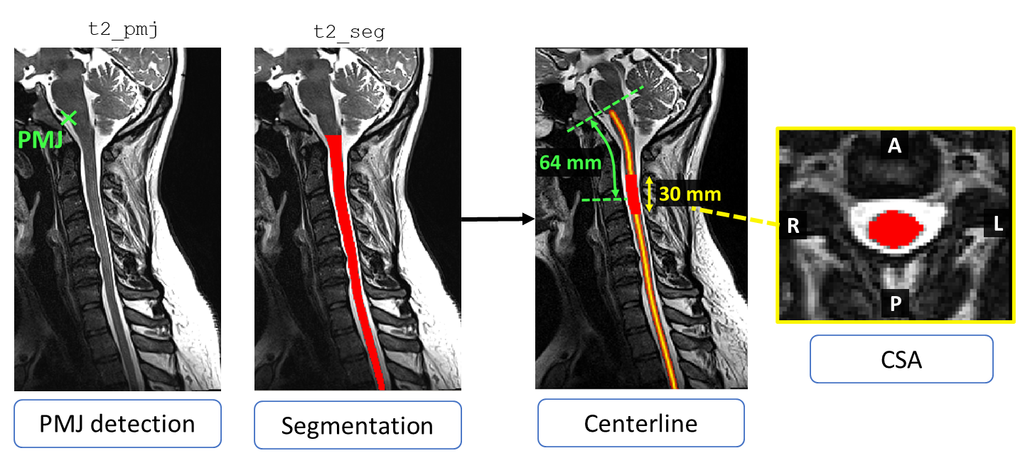
PMJ-based CSA at 64 mm using a 30 mm extent mask.
PMJ detection
First, we proceed to the detection of the PMJ.
sct_detect_pmj -i t2.nii.gz -c t2 -qc ~/qc_singleSubj
- Input arguments:
-i: Input image.-c: Contrast of the input image.-qc: Directory for Quality Control reporting.
- Output files/folders:
t2_pmj.nii.gz: An image containing the single-voxel PMJ label.
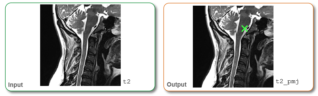
PMJ detection for T2.
CSA computation
Second, we compute CSA from a distance from the PMJ.
sct_process_segmentation -i t2_seg.nii.gz -pmj t2_pmj.nii.gz -pmj-distance 64 -pmj-extent 30 \
                         -o csa_pmj.csv -qc ~/qc_singleSubj -qc-image t2.nii.gz
- Input arguments:
-i: The input segmentation file.-pmj: The PMJ label file.-pmj-distance: Distance (mm) from the PMJ to center the mask for CSA computation.-pmj-extent: Extent (mm) for the mask to compute and average CSA.-o: The output CSV file.-qc: Directory for Quality Control reporting.-qc-image: Image to display as the background in the QC report. Here, we supply the source anatomical image (t2.nii.gz) that was used to generate the spinal cord segmentation (t2_seg.nii.gz).
- Output files/folders:
csa_pmj.csv: A file containing the CSA values and other shape metrics. This file is partially replicated in the table below.
Filename |
Slice (I->S) |
DistancePMJ |
MEAN(area) |
STD(area) |
|---|---|---|---|---|
single_subject/data/t2/t2_seg.nii.gz |
165:201 |
64.0 |
72.55544193058263 |
2.019934259168476 |
Note
The above commands will output the metrics in the subject space (with the original image’s slice numbers) However, you can get the corresponding slice number in the PAM50 space by using the flag -normalize-PAM50 1.
sct_process_segmentation -i t2_seg.nii.gz -discfile t2_totalspineseg_discs.nii.gz -perslice 1 -normalize-PAM50 1 -o csa_PAM50.csv